- Introduction
- Regularization
- Weight Initialisation
- Choosing Gradient Descent Parameters
- Activation Functions
- Loss Functions
- References
Introduction
I was part of the CVIT Summer School 2021, in one of the lectures by Prof.Vineeth Balasubramanian, the following slide was used to describe the various pieces which led to the advancements in DL.
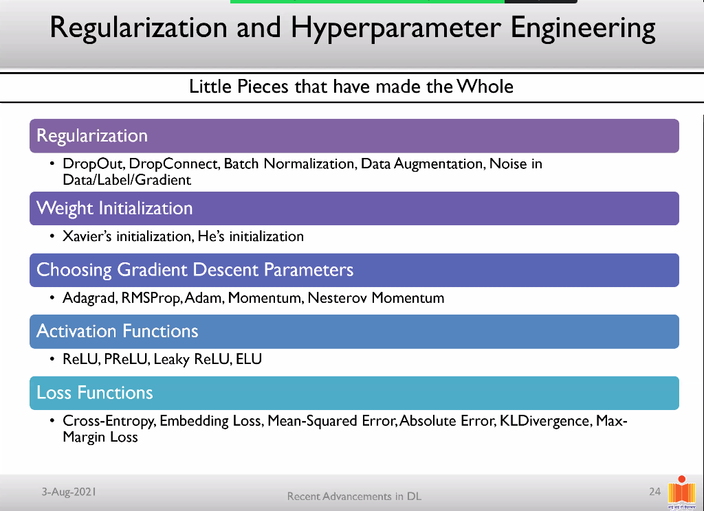
All the concepts mentioned in this slide are very important and the building blocks of a NN. These concepts are asked quite often in interviews, and I aim to write an overview of the concepts mentioned here for a quick glance and revision.
Regularization
Regularization is the concept of adding an additional term or penalty to your loss function such that it makes the model harder to learn the existing concept. It is often a common method used to solve the problem of overfitting since the weight added slows the weight update process and makes it harder to learn and not overfit.
1. Dropout
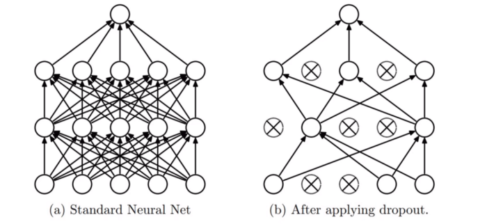
Dropout is a commonly used method in deep learning. In Dropout, you randomly drop a set of neurons in your neural network based on a probability metric. So the network is made to learn with a lesser number of neurons or weights which makes it learn better, more robust, and not overfit on the data.

- Dropout drops the activations in the network.
- Dropout is used only in the training process and not during test time.
2. DropConnect

DropConnect is similar to Dropout, but it drops the weights instead of the nodes in the network with a certain probability, so a node remains partially active.
Both Dropout and DropConnect are methods used to prevent co-adaption in the network. This means that we want the units to independently learn rather than depending on each other. In each training step, the weights or activations drop will be different.
3. Batch Normalization
In Batch Normalization(BN), we take the average of the mean and standard deviations of the activations of the layers and use these to normalize the activations. This way the distribution of the neurons after each layer remains the same, thus boosting the performance of the model, speeds up training, and gives us the ability to use a higher learning rate.
BN is applied for every training mini-batch. It is believed that BN adds a sense of randomness since each mini-batch will have a different set of means and standard deviations, thus the normalized values will be slightly different each time.

- If the normalized activations are y^. BN Layer would contain: gamma * y^ + beta, where gamma, beta are learnable parameters. These are used to tune the normalized activations to make accurate predictions.
4. Data Augmentation
Data augmentation is the process of :
- adding variety to your dataset by having variations to your data,
- helps in increasing your dataset size.
- helps in making the model more robust and prevents overfitting to some extent.
Examples of common data augmentation techniques for images are rotation, flipping, perspective warping, brightness changes, and contrast changes. Examples for text include back translation, synonym replacement, random insertion etc.
5. Noise in Data/Label/Gradient
It has been observed that adding random noise helps in generalisation, fault tolerance, and better learning. Adding noise has a regularization effect.
The ways we can add noise include:
- adding noise to training data ( a form of data augmentation )
- adding noise to labels ( class labels )
- adding gradient noise

Gaussian noise is added to every gradient g at every time step t.
Weight Initialisation
Weight initialisation is the concept of how the weights in the model are initialised before the training is started. It plays a huge impact on how well the model learns and has an effect on the final accuracy as well.
1. Xavier’s initialisation
The goal of this intialisation is to ensure that the variance of activations is the same across all layers. The constant variance helps in avoiding the gradient from exploding or vanishing.
- Xavier init is designed to work well with tanh and sigmoid activations.
Xavier initialization sets a layer’s weights to values chosen from a random uniform distribution that’s bounded between :

In the above equation:
- nj is the number of incoming connections to a layer.
- nj+1 is the number of outgoing connections from a layer.
2. He’s initialisation
This is more suited for activation functions such as ReLU, it takes into account the non-linearity of functions.
 It draws samples from a truncated normal distribution centered on 0 with stddev = sqrt(2 / fan_in) where fan_in is the number of input units in the weight tensor.
Choosing Gradient Descent Parameters
We discuss the optimizers are used in the gradient descent process. These help in training the network better and reaching the global minima faster.
1. Adagrad : Adaptive Gradient Optimizer
w' = w - alpha * dw
Typically in GD, mini-batch GD, the learning rate is fixed.
Core idea : each weight has a different learning rate. It is parameter-based learning rate tuning.
- More updates a parameter gets, smaller the weightage of the update. [low learning rate for parameters of frequently occurring features]
- Fewer updates a parameter gets, more the weightage of the update. [high learning rate for parameters for infrequently occurring features]
It is well suited for working with sparse data.

where Gt holds the sum of the squares of all previous gradients till the point t.
Advantages :
- No need to manually change the learning rate.
Disadvantages :
- Accumulation of squared gradient in the denominator. It keeps increasing with training and thus leads to making the learning rate too small with time.
2. RMSProp - Root Mean Squared
It is very similar to Adagrad but it aims to fix the problem of the diminishing gradient by using an exponentially decaying average of the gradient.
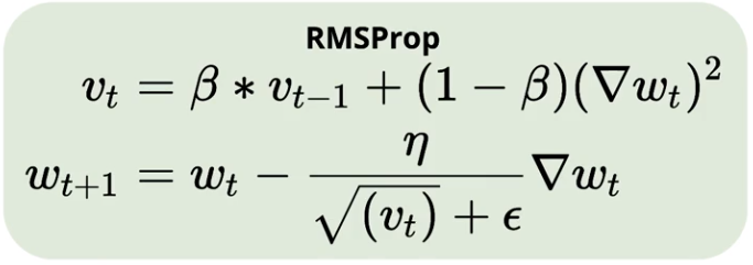
For example, in the above equation
- if value of beta = 0.9,
- vt will be 0.9 * previous gradient + 0.1 * (current_gradient) ^ 2
This means the direction of the previous gradients is given more weightage than the recent update. This ensures that the gradient does not oscillate much and moves in the right direction.

3. Adam - Adaptive Moment Estimation
The addition in Adam is that it stores :
- exponentially decaying average of past gradients (mt) - Equation 1 +
- exponentially decaying average of past squared gradients (vt) - Equation 2 [As in RMSProp]
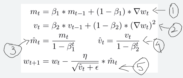
The authors observed that when :
- mt, vt are initialised as vectors of zeros and
- when B1, B2 are small ( close to 1)
- mt, vt were biased towards zeros
To counter these biases, they compute bias-corrected moments i.e equation 3 and 4 in the above figure.
Equation 5 is the final Adam equation.
Authors propose the following default values :
- B1 - 0.9
- B2 - 0.999
- Epsilon - 10^-8
- Good default suggested for Learning rate - n - 0.001
According to Kingma et al., 2014, the Adam optimizer is “computationally efficient, has little memory requirement, invariant to diagonal rescaling of gradients, and is well suited for problems that are large in terms of data/parameters”.
4. Momentum
Momentum helps in reaching the minima faster by giving a push by making the gradient move in the direction of the previous update. It results in faster convergence and reduced oscillations.
Equation : w = w - n * dw + gamma * vt
    where n - the learning rate
          vt - is the value of w at time t-1 (last update to w)
          gamma - the momentum parameter (usually initialised to 0.9)
This gist of momentum is that we get to local minima faster because we don’t oscillate up and down the y-axis. The time to convergence is faster when using momentum.
Pros :
- faster convergence than SGD Cons :
- If momentum is too high, then we may miss the minima and move ahead, then moving backwards and end up missing it again.
5. Nesterov Momentum (look-ahead momentum)
It is a kind of look-ahead momentum updation. This is done by using an approximation of the next gradient value in the present momentum update equation.
w_ahead = w + gamma * vt-1 [n*dw is ignored]
(Gives an approximation of the next position of parameters, refer momentum eq.)
vt = gamma * vt-1 - n * dw_ahead
w = w + vt
The gradient is computed at the lookahead point(w_ahead) instead of the old position w.

Nesterov momentum: Instead of evaluating the gradient at the current position (red circle), we know that our momentum is about to carry us to the tip of the green arrow. With Nesterov momentum, we therefore instead evaluate the gradient at this “looked-ahead” position.
Activation Functions
An activation function is a non-linear transformation we do over the weighted sum of inputs before sending it to the next layer.
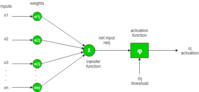
Activation functions add non-linearity to our NN and without it, our NN would just be a product + bias addition which would be a linear transformation. This would limit the capabilities of our NN.
1. ReLU - Rectified Linear Unit
ReLU function :
  f(x) = 0 , x < 0
       = x when x > 0
  -> f(x) = max(0, x)
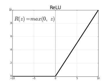
ReLU helps in faster and efficient training of the NN and leads to fewer vanishing gradient problems.
Issues :
- Non-differentiable at zero.
- Not zero-centered
- Unbounded
- Neurons can be pushed into states in which they become inactive for essentially all inputs. This is called the dying ReLU problem.
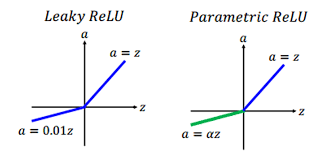
2. Leaky ReLUs
Modified version of ReLU
  f(x) = x , when x > 0
       = 0.01 * x, when x < 0
Leaky ReLUs allow a small, positive gradient when the unit is not active. This activation is preferred in tasks that suffer from sparse gradients, for example in training GANs.
3. PReLU - Parametric ReLU
The generalized version of Leaky ReLU, where a parameter is used instead of 0.01.
Parametric ReLU
  f(x) = x , x > 0
         alpha * x, x < 0
Alpha is learned along with other NN parameters. The intuition is that different layers may require different types of non-linearity.
4. ELU - Exponential Linear Units
ELU function :
    f(x) = x , x > 0
           a*(e^x - 1) , otherwise
  a is a hyperparameter to be tuned, and a > 0 is a constraint.
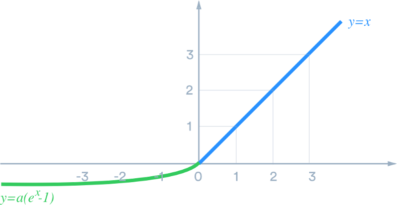
ELUs try to make the mean activations closer to zero, which speeds up the learning.
Loss Functions
A loss function is a function we use to optimize the parameters of our model.
1. Cross Entropy Loss
It is generally used for the optimization of classification problems. When the number of classes is 2, it is known as binary cross entropy loss.

2. Embedding Loss
The embedding loss functions are a class of loss functions used in deep metric learning. These are used to improve the embedding generated so that similar inputs have a closer distance and dissimilar inputs have a larger distance. Examples of embedding losses are contrastive loss, triplet loss, margin loss etc.
3. Mean-Squared Loss
The average squared error of the actual and estimated value i.e mean of the square of the errors.

It is a commonly used loss function for regression.
4. Absolute Error
The sum of the absolute difference between the actual and estimated value.
  Absolute Error : |y-y_|
           where y is the actual value
                 y_ is the estimated value
It is a loss function used to regression models
5. KLDivergence
It is the measure of how two probability distributions (eg: p and q ) are different from each other.
  KLDivergence :
    D(P || Q) = summation p(x) * log(p(x)/q(x))
As a loss function, the divergence loss between y_true and y_pred is calculated.
Loss(y_true || y_pred) = y_true * log(y_true/y_pred)
6. Max-Margin Loss
It is also known as hinge loss. It is used for training SVMs for the task of classification.
  Loss = max(1 - y_true * y_pred, 0)
  y_true are expected to be -1 or 1.
References
In writing this post, I have referred various articles, blog posts, the FastAI book to get a better understanding. I am adding some references to read deeper on some of the topics :
- Optimizers :
- Embedding Loss :
- Explanation of the various embedding loss functions - Link
- FastAI Book - Link
Do comment and let me know if you have any feedback or suggestions to improve this blogpost. Thank you!